
Analysis of Particle Size Distribution D10/D50/D90
Analysis particle size distribution is crucial for quality control and research, as it directly impacts various material properties. These properties include flow characteristics, reactivity, abrasiveness, solubility, extraction efficiency, taste, compressibility, and more.
Particle size distribution analysis is a standard practice in laboratories, employing various techniques depending on the material and examination goals. Common methods include Laser Diffraction (LD), Dynamic Light Scattering (DLS), Dynamic Image Analysis (DIA), and Sieve Analysis. These techniques are typically used for suspensions, emulsions, and bulk materials, with aerosols being analyzed in rare cases.
Methods for Determining Particle Size Distribution
Most samples are typically polydisperse systems, meaning they consist of particles of various sizes rather than a uniform size. Particle size distribution describes the proportion of particles that fall within specific size intervals, often referred to as size classes or fractions.
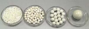
For example, consider a mixture of grinding balls sorted by size: 5 mm, 10 mm, 15 mm, and 40 mm. This illustrates how the distribution can provide insights into the variety of sizes present in a sample.
Quantification Methods for Particle Size Distribution
Quantification of particle size distribution can be accomplished in several ways:
- Weighing: Each size fraction may contain 190 g of sample, representing 25% of the total weight. This mass distribution correlates with volume distribution, assuming density remains constant across particle sizes.
- Counting: The total sample consists of 573 particles distributed among the four size fractions. For instance, there is only one sphere measuring 40 mm, accounting for just 0.2% of the total count, despite representing 25% by weight. Conversely, the 490 spheres with a diameter of 5 mm make up 85.5% of the total number.CEP
These different methods—counting versus mass/volume—can yield significantly different particle size distributions for the same sample.
Particle size analyzers may provide distributions based on numbers (as seen in Dynamic Image Analysis), mass (from Sieve Analysis), or volume (using Laser Diffraction). With appropriate modeling, these distributions can often be converted between one another. A notable exception is Dynamic Light Scattering, which typically reports intensity-based particle size distributions. In this case, larger particles dominate the representation, as scattering intensity decreases with size by a factor of 10^6.
Presentation of Particle Size Distribution Results
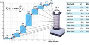
Particle size distribution can be presented in either tabular or graphical formats. The table below illustrates the distribution for the grinding balls, where P0P_0P0 indicates number-based quantities and P3P_3P3 denotes mass or volume-based quantities.
| Size | Weight P3P_3P3 | Percentage | Number P0P_0P0 | Percentage |
| 5 mm | 190 g | 25% | 490 | 85.5% |
| 10 mm | 190 g | 25% | 64 | 11.2% |
| 15 mm | 190 g | 25% | 18 | 3.1% |
| 40 mm | 190 g | 25% | 1 | 0.2% |
| Total | 760 g | 100% | 573 | 100% |
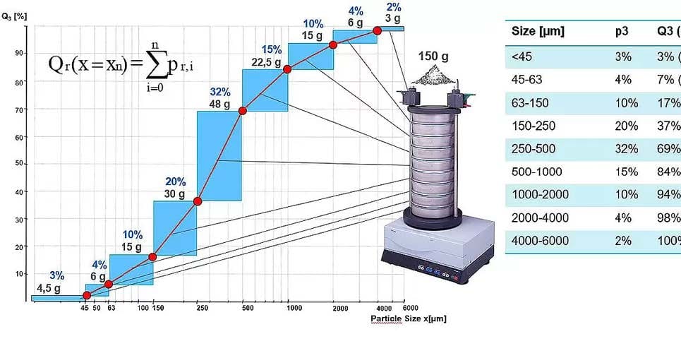
A descriptive method to represent particle size distribution is through a histogram. In this graph, the width of each bar represents the size class limits, while the height reflects the quantity within that class.
In particle measurement technology, it is common to generate a cumulative distribution based on the class-dependent values. This involves summing the quantities in each measurement class, starting from the smallest size fraction, resulting in a cumulative curve that increases continuously from 0% to 100%. This cumulative curve is denoted as QQQ. Each value Q(x)Q(x)Q(x) represents the portion of the sample made up of particles smaller than size xxx. Since this corresponds to the amount that would pass through a hypothetical sieve of mesh size xxx, it is often referred to as “percent passing.”
Occasionally, the fractions are summed from the largest particle size downwards. This yields a curve that declines from 100% to 0%, known as the 1−Q1-Q1−Q distribution. This distribution indicates the percentage of the sample larger than size xxx and is termed “percent retained,” as it reflects how much of the total sample would be retained by a particular sieve.
Parameters Derived from Particle Size Distribution Analysis
A variety of statistical parameters can be extracted from particle size distribution data, with the cumulative distribution being particularly useful for this purpose. Among the key parameters are percentiles, which indicate the particle size xxx below which a certain percentage of the sample lies. For example, they can answer questions such as “What size do the 10% smallest particles fall below?” or “What size do the 5% largest particles exceed?” Percentiles can be directly read from the cumulative QQQ or 1−Q1-Q1−Q curves.
Percentiles are denoted by the letter ddd followed by the percentage value. For instance, d10=83 μmd_{10} = 83 \, \mu md10=83μm, d50=330 μmd_{50} = 330 \, \mu md50=330μm, and d90=1600 μmd_{90} = 1600 \, \mu md90=1600μm indicate that 10% of the sample is smaller than 83 μm, 50% is smaller than 330 μm, and 90% is smaller than 1600 μm. Alternative notations include x10/50/90x_{10}/50/90×10/50/90 or D0.1/0.5/0.9D_{0.1}/0.5/0.9D0.1/0.5/0.9. The d50d_{50}d50 value, also known as the “median,” divides the distribution into equal halves of smaller and larger particles.
Typically, d10d_{10}d10, d50d_{50}d50, and d90d_{90}d90 are reported for a particle size distribution. This trio of values provides a clear characterization of the distribution’s central point as well as its upper and lower extremes. While this approach is generally effective, it may not always capture all relevant information. Additional percentiles, such as d16d_{16}d16, d84d_{84}d84, d95d_{95}d95, and d99d_{99}d99, can also be defined.
It’s important to consider whether the measurement method is sensitive enough to accurately detect percentiles close to 0% or 100%. The d100d_{100}d100 value is often ambiguous and not clearly defined; for example, if 100% of particles are less than 2 mm, this holds true for all larger size values, making the d100d_{100}d100 value less meaningful.
Mean Values and Distribution Characteristics in Particle Size Analysis
Mean values, or mean particle size, can be calculated from tabulated data by multiplying the quantity in each measurement class by the mean size of that class and then summing these products. Several methods for calculating the mean are outlined in ISO 9276-2.
To describe the width of the distribution, the standard deviation around the mean can be utilized, along with the span value, which is calculated as (d90−d10)/d50(d_{90} – d_{10}) / d_{50}(d90−d10)/d50. A wider distribution will result in a larger standard deviation and span.
The size at which the density distribution reaches its maximum, known as the mode size, indicates the most frequently occurring measurement class. Particle size distributions that exhibit multiple peaks in the density distribution are termed multimodal (or bimodal, trimodal, etc.).
A key consideration in particle size distribution analysis is identifying oversize and undersize particles. These are small fractions of particles that are significantly larger or smaller than the majority of the sample. In the cumulative curve, oversize or undersize particles are indicated by a step, while in the density distribution, they may appear as a secondary peak outside the main distribution.
For instance, consider a particle size distribution with 5% oversize, where 95% of the particles are below 1 mm, and the oversize particles range from 1 to 1.25 mm. This can be quantified with Q3(1 mm)=95%Q_3(1 \, \text{mm}) = 95\%Q3(1mm)=95% or 1−Q3(1 mm)=5%1 – Q_3(1 \, \text{mm}) = 5\%1−Q3(1mm)=5%. The presence of oversize particles will increase the mean particle size, while the median remains unaffected. Alternatively, the effect of oversize can also be reflected in an increased d95d_{95}d95.
Analysis of Particle Size Distribution – FAQ
What is Particle Size Distribution?
Particle Size Distribution (PSD) refers to the frequency of particles of different sizes in a sample of powder, granulate, suspension, or emulsion. It represents a statistical concept, typically expressed as percentages for specific size intervals (fractions) or as cumulative values that sum fractions in ascending or descending order.
Which methods are used to measure Particle Size Distribution?
There are various methods to determine PSD, with the choice depending on the particle size range and material properties. Common techniques include sieve analysis, laser diffraction, dynamic light scattering, and image analysis.
Why is Particle Size Distribution important?
PSD is a critical quality parameter for many products and raw materials, as it influences various material properties. Key factors affected by PSD include flowability, surface area, conveying characteristics, extraction and dissolution behavior, reactivity, abrasiveness, and even taste.
What do d10, d50, and d90 mean in Particle Size Distribution?
d10, d50, and d90 are percentile values that can be directly derived from the cumulative particle size distribution. They represent the sizes below which 10%, 50%, and 90% of the particles fall, respectively.
What is the difference between monomodal and bimodal Particle Size Distribution?
The mode size is where the frequency distribution peaks. A distribution with a single peak is called monomodal, while one with two peaks is termed bimodal. Distributions with more than two peaks are referred to as multimodal.
How is the width of a particle size distribution specified?
The width of a particle size distribution is an important statistical characteristic. A distribution is called monodisperse when all particles are of the same size, whereas polydisperse systems contain particles of varying sizes. The width can be quantified using the standard deviation around the mean particle size or by calculating (d90−d10)/d50(d_{90} – d_{10}) / d_{50}(d90−d10)/d50.