
Overview of statistical concepts-Bioequivalence Pharmacokinetics
INTRODUCTION
Overview-of-statistical-concepts-bioequivalence, Current global regulatory agencies mandate that the final assessment of an oral medication’s quality relies on its in vitro dissolution behavior, along with in vivo bioavailability and/or bioequivalence evaluations. The latter hinges on the assumption that the drug concentration in systemic circulation equates to its concentration at the site of action, and that the drug’s therapeutic effect is governed by its pharmacodynamic-pharmacokinetic relationship.
Bioequivalence has garnered increasing attention over the past four decades due to the realization that different products with equal drug quantities may elicit varying therapeutic responses, often attributable to differences in drug plasma levels stemming from absorption issues. Numerous instances in the literature, such as correlations between bioavailability and clinical efficacy of various drugs, underscore this phenomenon. Substantial evidence now suggests that drug response correlates more strongly with plasma concentration or drug quantity in the body than with the administered dose alone. Consequently, bioavailability and bioequivalence studies, grounded in basic pharmacokinetic principles and parameters, serve as viable alternatives to costly and complex clinical trials, widely employed globally to ensure consistent quality and reliable therapeutic performance of marketed medications.
Bioavailability indicates the systemic availability of the active therapeutic component, typically assessed through parameters like the area under the concentration-time curve (AUC), peak plasma concentration (Cmax), and time to reach Cmax (Tmax). It depends on factors such as drug absorption from the administration site, the drug itself, the dosage form, and their interaction with the absorption site environment. In linear pharmacokinetics, AUC and Cmax values increase proportionally with the dose, allowing comparison of systemic availability between different formulations. However, for drugs following non-linear kinetics, where processes like absorption, distribution, metabolism, or excretion become saturated within the therapeutic concentration range, assessing absolute bioavailability requires measuring drug and metabolite excretion in urine.
Bioequivalence evaluation compares the rate and extent of absorption of multiple drug formulations with an innovator (reference) product, assuming similar concentration-time profiles in blood/plasma correspond to similar therapeutic effects. For generic products to be accepted as therapeutically equivalent to the innovator, they must establish bioequivalence in vivo. These studies also serve as quality control measures for production and manufacturing changes. Bioequivalence studies are mandated in three scenarios: when the proposed dosage form differs from that used in pivotal trials, significant changes occur in the formulation’s manufacturing, or when a new generic formulation is compared to the innovator product.
The design, execution, and assessment of bioequivalence studies have garnered significant attention from academia, pharmaceutical industry, and regulatory bodies over the past two decades. This article aims to provide an overview and delve into the evolution and synthesis of key statistical analysis concepts applied in bioequivalence studies.
STUDY DESIGN CONCEPTS: Overview-of-statistical-concepts-bioequivalence
According to guidelines set forth by the US FDA (1992), most bioequivalence trials typically involve comparing a “test” formulation with a standard/innovator “reference” formulation among a group of healthy subjects aged 18-55. Each subject receives both treatments alternately in a crossover fashion, with treatments separated by a “washout period” usually lasting a week, though it may be longer if the drug’s elimination half-life is prolonged. This randomization also applies to three-treatment crossover designs.
Many drugs exhibit significant inter-subject variability in clearance, with intra-subject coefficient of variation typically smaller than between subjects. Consequently, crossover designs are often preferred for bioequivalence studies due to their ability to mitigate intersubject variability. The primary advantage of the crossover design lies in comparing treatments within the same subject, thereby minimizing error variability attributed to intersubject differences. However, in cases where the drug or its metabolites have an extended half-life, a parallel group design may be more appropriate. In a parallel group design, subjects are randomly assigned to receive only one treatment, thus necessitating a larger sample size compared to crossover designs to maintain sensitivity.
Both crossover and parallel designs adhere to three key statistical concepts:
randomization, replication, and error control. Randomization ensures unbiased allocation of treatments to subjects, essential for obtaining accurate treatment effect estimates. Replication involves applying treatments to multiple experimental units to enhance the reliability of estimates and provide a more precise measurement of treatment effects. Sample size for replication depends on the degree of differences to be detected and inherent data variability. Replication is coupled with error control to minimize experimental error or error variability.
(ANOVA) ANALYSIS OF VARIANCE-Overview-of-statistical-concepts-bioequivalence
Pharmacokinetic parameters such as AUC and Cmax, obtained from the plasma concentration-time curve, undergo ANOVA to partition variance into components attributed to subjects, periods, and treatments. The traditional null hypothesis assumes equal means (H0: µT = µR) signifying bioequivalence, where µT and µR denote the expected mean bioavailabilities of test and reference formulations, respectively. Conversely, the alternate hypothesis (H1: µT ≠ µR) suggests bioinequivalence. For crossover trials involving n subjects and t treatments, ANOVA assumes a specific structure. Anova Calculation Full Excel.
How error variability in ANOVA is contingent on study design. Consider comparing two treatments, T1 and T2, with a group of subjects. Two experimental designs emerge: (i) Parallel Group Design allocates each treatment to a separate subject group; (ii) Crossover Design treats each subject as a block, administering both treatments on distinct occasions. While parallel design isolates variability due to treatment, crossover design separates out variability due to treatment, subject, and period. Consequently, the error sum of squares (SSE) in parallel design surpasses that of crossover design for a given sample size. Although the degrees of freedom for SSE remain consistent across designs (for the two-treatment scenario), the error mean sum of square (MSE) is greater in parallel design than in crossover design. This implies greater error variability in parallel group design compared to crossover design.
ANOVA compares the mean sum of squares attributed to a factor with that of error (e.g., F = MST / MSE). If these sums are comparable, no difference between in factor levels is inferred; otherwise, a difference is concluded. Should a difference exist in treatments, i.e., treatment mean sum of squares exceeds error mean sum of squares, Design 2 is more likely to detect this difference than Design 1, given that MSE2 < MSE1. This underscores Design 2’s greater statistical power compared to Design 1, highlighting how experimental design influences test power.
In bioequivalence studies, the F-statistic compares formulations’ mean sum of squares to error mean sum of squares to test H0: µT = µR. However, testing this simple null hypothesis is of little interest as formulations’ mean drug absorption amounts aren’t expected to be identical due to various factors.
Instead, interest lies in assessing whether the difference between treatments falls within a predefined margin, typically 20% of the reference mean.
Addressing these complexities, bioequivalence determination adopts two approaches: hypothesis testing and estimation via confidence intervals.
APPROACH HYPOTHESIS TESTING Overview-of-statistical-concepts-bioequivalence
When employing statistical hypothesis testing, it’s crucial to articulate the hypothesis accurately. In this paradigm, the hypothesis intended for validation is formulated as the alternative hypothesis. The null hypothesis is rejected in favor of the alternative if the evidence strongly opposes the null. Hauck and Anderson (1984) proposed incorporating the objective of bioequivalence trials into interval hypotheses, with the allowable range denoted as Δ:
H0: Products are bio inequivalent
H1: Products are bioequivalent
They provided a test statistic for this hypothesis. However, it was noted that when degrees of freedom are low, the actual significance level exceeds the nominal level (α), resulting in a consumer’s risk greater than 5%. Consequently, this approach didn’t gain traction in bioequivalence testing methodology.
In 1987, Schuirmann introduced the two one-sided t-tests procedure for bioequivalence. This method decomposes the interval hypothesis 0H0 into two sets of one-sided hypotheses and applies two separate t-tests:

H01:μT−μR≤−Δ(Lower bound)
H02:μT−μR≥Δ(Upper bound)
The null hypotheses (H01 and H02 ) of bioequivalence are rejected if:
s/nxˉT−xˉR>t1−α/2(v)ors/nxˉT−xˉR<−t1−α/2(v)
where s is the square root of the mean square error from the crossover design ANOVA, n is the number of subjects per period, and t1−α/2(v) is the critical value of 1−α/2 in the upper tail of the Student’s t-distribution with degrees of freedom v.
Remarkably, the current FDA guidelines lack explicit mention of power. Reframing the
hypothesis as
H0:Products are bioequivalent
and
H1:Products are bioequivalent
leads to:
α=Probability [Reject H0 when H0 is true]
= Probability [Conclude bioequivalence when products are bioinequivalent]
=Probability [Conclude bioequivalence when products are bioinequivalent]
=Consumer’s risk=Consumer’s risk
β=Probability [Accept H0 when H0 is false]
=Probability [Conclude bioinequivalence when products are bioequivalent]
=Probability [Conclude bioinequivalence when products are bioequivalent]
=Manufacturer’s risk=Manufacturer’s risk.
Power=1−β
The roles of α and β are thus interchanged. With α set at 0.05, constraining the consumer’s risk to 5%, the FDA leaves it to the pharmaceutical industry to determine the extent of the manufacturer’s risk.
Therefore, in the FDA’s guidelines, power is not explicitly addressed, but adequate sample size can minimize the manufacturer’s risk.
APPROACH CONFIDENCE INTERVAL
Westlake 24 was the first to propose the utilization of confidence intervals (C.I.) as a method to assess bioequivalence, determining whether the mean drug absorption with a test formulation closely aligns with that of a reference. The fundamental concept of a confidence interval (C.I.) and its interpretation
comes to the forefront. For instance, a 95% C.I. for the difference in AUC’s (area under the curve) between test and reference formulations can be calculated using specific equations and critical values.
This C.I. implies a 95% confidence level that the true difference lies within the calculated limits, known as the lower and upper confidence limits. The confidence level, often set at 95%, expresses the precision of the estimated statistic. A narrower C.I. indicates increased precision, typically achieved by reducing variability or standard error.
Various scholars, including Westlake24, Metzler25, and Kirkwood26, proposed constructing C.I.s for bioequivalence testing, typically with a significance level (a) set at 0.05. The decision-making process often involves accepting bioequivalence if the C.I. falls within predetermined bioequivalence ranges.
However, early methods had limitations, prompting refinements over time.
In 1981, Westlake28 sought to align the acceptance criteria for bioequivalence with established principles for efficacy trials, where a significance level of a=0.05 is common. This alignment led to the proposal of using a 90% C.I. instead of the traditional 95% C.I., aiming to balance the risks of both type I
and type II errors.
Adopting a 90% C.I. is equivalent to rejecting both null hypotheses at the nominal a (=0.05) level through two one-sided t-tests. Although both approaches hold similar implications, they are often simultaneously employed in practice.
BIOEQUIVALENCE PARAMETERS to LOGARITHMIC
TRANSFORMATION
Bioequivalence studies evaluate and compare key parameters such as AUC, Cmax, and Tmax of
different formulations. Regulatory guidelines advise logarithmic transformation of AUC and Cmax prior to statistical analysis for several reasons.
Firstly, from a clinical standpoint, the primary focus lies in comparing the ratio rather than the difference between average parameter data of test and reference formulations. Log transformation facilitates this comparison statistically.
Secondly, in terms of pharmacokinetics, while the crossover design assumes additive effects due to subject, period, and treatment, pharmacokinetic equations operate multiplicatively. Logarithmic transformation converts these equations into additive models, aiding in analysis.
Additionally, log transformation addresses the statistical aspect by aligning data more closely with a log-normal distribution, especially since AUC and Cmax often exhibit skewed distributions with variance dependent on the means.
Regarding Tmax, its discrete nature and measurement error pose unique challenges. While some suggest confidence intervals based on untransformed data, regulatory agencies prefer non-parametric tests for evaluating differences in Tmax.
In essence, logarithmic transformation enhances the interpretation and analysis of bioequivalence study data, ensuring robust comparisons between formulations.
RANGE of BIOEQUIVALENCE
The US FDA employs an equivalence range of 80-120% for the 90% confidence interval (C.I.) of the ratio of product averages as a standard criterion for various drugs when analyzed on the original scale. This range allows for a relative difference between product averages of ±20%. It’s crucial to designate one
product as the reference to maintain consistency, as swapping their roles can alter the conclusion of equivalence.
When analyzing log-transformed data for parameters like AUC and Cmax, it’s recommended to utilize an equivalence criterion of 80-125% for the 90% C.I. of the ratio of product averages. This wider range offers an advantage over the 80-120% criterion, as it maximizes the probability of concluding bioequivalence
when the ratio of averages is exactly 1. Unlike the 80-120% range, the 80-125% range is symmetrically multiplicative, ensuring consistency regardless of the reference choice. Regulatory bodies generally prefer this wider criterion. However, for generic drug approval, this allows the test product to be up to
25% greater than the reference.
The CPMP guidance initially proposed an equivalence range of (0.70-1.43) for the C.I. of the Cmax ratio, but later revisions suggested that a wider range might be necessary for Cmax compared to AUC due to larger variation in single concentrations like Cmax. The choice of the appropriate bioequivalence range
may also depend on clinical considerations, with drugs having a narrow therapeutic range potentially requiring tighter limits, such as ‘0.9-1.11’ for the C.I. of the AUC ratio and ‘0.8-1.25’ for the C.I. of the Cmax ratio. The US FDA maintains the ‘0.8-1.25’ range for the C.I. of the ratio (for log-transformed data) concerning Cmax, while the Canadian Health Protection Branch considers the range ‘0.8-1.25’ for the point estimate.
Regulatory standard for assessing
bioequivalence
The current regulatory standard for assessing bioequivalence involves analyzing data using logarithmic transformation for Cmax and AUC. Bioequivalence is determined if the 90% confidence interval (C.I.) for the ratios of the bioavailabilities of two formulations falls within the specified bioequivalence range [d1=0.80, d2=1.25]. The 90% C.I. for the ratio is calculated using the formula Exp, where s represents the square root of the Mean Square Error (MSE) from the crossover design ANOVA, n is the number of subjects per period, t0.05(1) denotes the critical value of t at a = 0.05, and v signifies the degrees of freedom associated with the MSE. Alternatively, bioequivalence can also be established when both sides of Schuirmann’s t-test yield statistically significant results (P < 0.05).
Sample size
In terms of sample size determination, as per the CPMP guidance, the required number of subjects depends on the error variance associated with the primary characteristic under study (estimated from pilot experiments, previous studies, or published data), the desired significance level, the expected deviation from the reference product, and the desired power. It is recommended to calculate the sample size using appropriate methods, ensuring it is not less than 12 subjects. The equations for approximate sample size calculation for the two one-sided ‘t’ tests, based on the additive model (untransformed data), are provided below (given that power curves are symmetric, the formulae are presented solely for δ > 0): [Insert Liu and Chow’s equations for sample size calculation here].
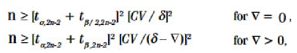
In this equation, where ‘n’ represents the number of subjects per sequence, ‘CV’ denotes the coefficient of variation, and ‘d’ stands for the bioequivalence limit.
This formula can be understood as follows:

(i) The minimum detectable difference between population means: Detecting a very small difference necessitates a larger sample size compared to detecting a large difference.
(ii) Population variance, represented by CV: If there is significant variability within samples, a larger sample size is needed to effectively detect differences between means.
(iii) The significance level ‘α’: When the test is conducted at a lower significance level, the critical value ‘ta,v’ will be higher, requiring a larger sample size to achieve the desired ability to detect differences between means. In other words, if there is a desire for a low probability of committing a Type I error (i.e., falsely rejecting H0).
